Dynamically Assisted Schwinger Effect

This document was made in parallel to my understanding of Schwinger pair production and the dynamically assisted Schwinger effect.

Unless stated otherwise, I use natural units ( $\hbar=c=1$ ).

Nothing here is to be taken as a scientific source of truth.

This is just my understanding, with the analogies and visualizations that helped me make sense of it.

Introduction

My previous writeup discussed the Schwinger model—the continuum and lattice model, its Hamiltonian, and the introduction of an external electric field.

This document explores an interesting phenomenon related to the Schwinger model: the Schwinger effect, where electron-positron pairs can be created from the vacuum by an external electric field.

A distinction worth keeping in mind throughout this document: the Schwinger model is QED in $1+1$ dimensions, whereas the Schwinger effect is the pair-production mechanism. They are closely related, but they are not the same thing. Some of the calculations below treat the electric field as an externally prescribed background instead of solving the fully dynamical gauge theory.

Recap—What is the Schwinger Model?

The Schwinger model asks what happens when light and electrons interact in a universe with one space dimension. It is a $1+1$ D system—1 space and 1 time dimension.

A quantum fermionic field $\psi(x,t)$ exists everywhere in the universe. This field can create and annihilate fermions and antifermions.

An electromagnetic gauge field $A_\mu(x,t)$ also exists. In one spatial dimension, the electromagnetic field has only one independent field-strength component: the electric field.

The massive Schwinger model is described by the Lagrangian

$$\boxed{\mathcal L=\bar\psi\left[i\gamma^\mu(\partial_\mu+ieA_\mu)-m\right]\psi -\frac14F_{\mu\nu}F^{\mu\nu}.}$$

Here, $\psi$ is the fermionic field, $A_\mu$ is the gauge field, $e$ is the coupling, $m$ is the fermion mass, and $F_{\mu\nu}$ describes the electric field. Setting $m=0$ gives the idealized massless Schwinger model discussed in my previous writeup 5.

One important feature of the $1+1$ D theory is that the electric field is tied directly to the charge density through Gauss's law. Schematically,

$$\partial_x E(x,t)=e\rho(x,t),$$

where $\rho$ is the charge density (the overall sign depends on the charge convention).

This will matter later. If an electron--positron pair is produced, the charges change the electric field around them. In the full Schwinger model, the gauge field responds to the produced particles; it is not just a background that sits there unchanged.

Why is pair production possible?

How can a vacuum, which supposedly contains no particles, produce particles?

To understand this, we first need to look at the energy spectrum of a free relativistic fermion. The relativistic wave equation for the electron was introduced by Dirac 1. Since the Schwinger model is $1+1$ D, we can work directly with a two-component Dirac spinor instead of starting with the four-component $3+1$ D version.

In natural units ( $\hbar=c=1$ ), a convenient momentum-space Dirac Hamiltonian is

$$H(k)=k\sigma_1+m\sigma_3,$$

where $k$ is the momentum, $m$ is the fermion mass, and $\sigma_1,\sigma_3$ are Pauli matrices. To find the energies, we solve the eigenvalue equation. Equivalently, we set the determinant of $H(k)-EI$ to zero:

$$\det\begin{pmatrix}m-E & k\\ k & -m-E\end{pmatrix}=0 \quad\Longrightarrow\quad E^2=k^2+m^2.$$

Therefore, the two energy branches are

$$\boxed{E_\pm(k)=\pm\sqrt{k^2+m^2}.}$$

The important part is that there are two energy branches: a positive-energy branch and a negative-energy branch.

At zero momentum,

$$E_+=+m,\qquad E_-=-m.$$

The two branches are separated by an energy gap of $2m$:

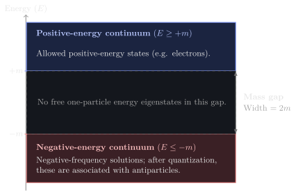
The diagram is a useful picture, but one detail matters: antiparticles are not simply the lower components of a Dirac spinor. In quantum field theory, particle and antiparticle operators are identified when the Dirac field is quantized. For now, we only need the existence of the two energy branches and the gap between them.

The Dirac-sea picture gives us a useful first intuition: promoting an occupied negative-energy state into the positive-energy sector leaves behind a hole, which we interpret as a positron. The promoted excitation is an electron, so the result is an electron--positron pair.

There is a more precise way to say this in quantum field theory (QFT). The Dirac field is not an ordinary wavefunction; it is an operator-valued field. When it is expanded in its positive- and negative-frequency solutions, the corresponding operators describe particles and antiparticles. Schematically,

$$\hat{\psi}(x)=\int dk\,\left[ \hat a_k u_k e^{-iE_kt+ikx} +\hat b_k^\dagger v_k e^{iE_kt-ikx} \right].$$

Here, $\hat a_k$ annihilates an electron and $\hat b_k^\dagger$ creates a positron. The vacuum is the state containing no electrons or positrons. The negative-frequency solutions are therefore not extra particles sitting inside the spinor; after quantization, they are associated with antiparticle creation. This is the standard QFT interpretation of the Dirac field 2.

The minimum energy needed to create a pair at rest is

$$\boxed{\Delta E=2m.}$$

So where does this energy come from? It can come from an external electromagnetic field, or, in the fully dynamical Schwinger model, from the energy stored in the gauge field. The field supplies energy to the fermionic degrees of freedom. There is no violation of energy conservation. We will return to the QFT meaning of a produced pair when we discuss time-dependent backgrounds and simulations.

How does pair production happen?

Introducing an external electric field

So far, we have considered a free fermion. Its Hamiltonian does not contain an electromagnetic field, so there is nothing that can transfer energy to the fermionic field or change its energy spectrum.

To introduce an electromagnetic background, we use minimal coupling. The momentum of a charged particle is shifted by the vector potential, and the scalar potential contributes a potential-energy term. In the $1+1$ D representation used above, the Hamiltonian becomes

$$H=\sigma_1(-i\partial_x-qA_x)+m\sigma_3+qA_0,$$

where $q>0$ is the magnitude of the fermion charge. For a static, uniform electric field, we can choose a gauge with $A_x=0$ and $A_0(x)=-Ex$. The potential energy is then

$$V(x)=qA_0(x)=-qEx.$$

This is a linear potential: the energy of a charge changes as it moves through the field. In other words, the electric field tilts the energy landscape. This is the starting point for understanding pair production through tunnelling.

Relativistic tunnelling

First, recall what tunnelling means in ordinary quantum mechanics. A particle may encounter a region where its energy is too small for classical motion. Its momentum would have to be imaginary there, so a classical particle cannot enter that region. A quantum wave, however, can extend into the region and emerge on the other side with a smaller amplitude. This is why a particle can sometimes pass through a barrier that it could not cross classically.

The Dirac equation has an extra feature: it has both positive- and negative-energy branches. An electric potential shifts the local energy of a charged fermion. For a state with conserved energy $\mathcal E$, the local relativistic energy--momentum relation is

$$(\mathcal E-V(x))^2=p(x)^2+m^2.$$

This is the free-particle relation $E^2=p^2+m^2$, but with the energy shifted by the potential. Rearranging gives

$$\boxed{p(x)^2=(\mathcal E-V(x))^2-m^2.}$$

Now we can identify where classical propagation is possible. If $p(x)^2\geq0$, the local momentum is real and the wave is oscillatory. If $p(x)^2<0$, the momentum is imaginary. Writing $p(x)=i\kappa(x)$ gives

$$\kappa(x)=\sqrt{m^2-(\mathcal E-V(x))^2}.$$

In this region the wave is exponentially varying rather than oscillatory. This is the forbidden region, and a quantum transition through it is tunnelling. Its boundaries, called turning points, occur when $p(x)=0$. Thus the forbidden region is where

$$-m<\mathcal E-V(x)<m.$$

This is the mass gap appearing locally in the presence of the potential. The important point is that the electric field changes where the positive- and negative-energy regions lie, and creates a region between them through which a transition can occur quantum mechanically.

A related idea is the Klein region. Consider a sufficiently large potential step. A positive-energy state on one side can overlap in energy with the negative-energy continuum on the other side if the potential difference exceeds the gap, $\Delta V>2m$. In a one-particle Dirac calculation this leads to the Klein paradox, first discussed by Oskar Klein 3. In QFT, the negative-energy channel is interpreted in terms of antiparticles, and the external field can produce particle--antiparticle pairs. The full scattering calculation is beyond what we need here. For our purposes, the Klein region shows how a strong potential can connect the two energy continua.

The Schwinger exponent

We now want to estimate how likely this tunnelling process is. The central idea of the WKB approximation is that the probability of crossing a forbidden region is controlled by how much the wavefunction is suppressed while it travels through that region. A wider or more strongly forbidden region gives a smaller transmission probability.

For a uniform electric field, $V(x)=-qEx$. The forbidden region is centered at a position that depends on $\mathcal E$, but shifting the origin of $x$ only moves the region; it does not change the tunnelling probability. We can therefore choose its center to be $x=0$ for the calculation. The magnitude of the imaginary momentum is then

$$|p(x)|=\sqrt{m^2-(qEx)^2},$$

with turning points

$$x_\pm=\pm\frac{m}{qE}.$$

In the WKB approximation, the leading tunnelling probability is the exponential of minus twice the integral of the imaginary momentum across the forbidden region:

$$P\propto\exp\left[-2\int_{x_-}^{x_+}|p(x)|\,dx\right].$$

The factor of two appears because the integral gives the suppression of the amplitude, while the probability is the squared amplitude. Substituting the momentum gives

$$P\propto\exp\left[-2\int_{-m/(qE)}^{m/(qE)} \sqrt{m^2-(qEx)^2}\,dx\right].$$

Use $u=qEx/m$. The integral becomes the area of a semicircle of unit radius:

$$\int_{-m/(qE)}^{m/(qE)}|p(x)|\,dx =\frac{m^2}{qE}\int_{-1}^{1}\sqrt{1-u^2}\,du =\frac{\pi m^2}{2qE}.$$

Therefore,

$$\boxed{P\propto\exp\left(-\frac{\pi m^2}{qE}\right).}$$

This is the leading exponential factor of Schwinger pair production 4, 10. The complete pair-production rate also contains a prefactor, but this exponent is enough to understand why the effect is difficult to observe.

It is useful to define a characteristic field strength, the Schwinger critical field:

$$\boxed{E_S=\frac{m^2}{q}.}$$

Restoring physical constants, $E_S=m^2c^3/(q\hbar)$. We can write the suppression as

$$P\propto\exp\left(-\pi\frac{E_S}{E}\right).$$

For $E\ll E_S$, the exponent is very large and negative, so pair production is exponentially suppressed. The critical field is not a strict threshold below which pair production is impossible. It is the characteristic scale at which the suppression becomes much weaker.

How can pair production be facilitated?

We have established that an electric field can produce pairs through tunnelling, but the probability is extremely small for subcritical fields. There are two useful ways to make pair production more effective:

1. Increase the strength of the electric field, making tunnelling easier.

2. Make the electric field time-dependent, allowing it to drive transitions between the energy branches.

The dynamically assisted Schwinger effect combines these two ideas.

Route I: a strong, slowly varying electric field

The first option is the one we have already encountered. Increasing $E$ makes the forbidden region narrower:

$$\Delta x=x_+-x_-=\frac{2m}{qE}.$$

It also decreases the exponent in $P\propto\exp(-\pi m^2/(qE))$. Both descriptions say the same thing: a stronger field makes tunnelling more likely.

The difficulty is the scale of the field required. For electrons, the Schwinger critical field is approximately

$$E_S\approx1.3\times10^{18}\ \mathrm{V/m}.$$

Reaching fields of this order is experimentally challenging. This motivates looking for another way to reduce the exponential suppression without simply increasing the field strength.

Route II: a time-dependent electric field

So far, the electric field has been static. Each momentum mode therefore has a time-independent Hamiltonian, and its energy is conserved. A time-dependent field changes the Hamiltonian itself. The external source can now exchange energy with the fermionic field.

For a spatially uniform electric field, choose the temporal gauge, where the scalar potential is zero:

$$A_0=0,\qquad E(t)=-\frac{dA_x(t)}{dt}.$$

Because the field is uniform in space, we can study each canonical momentum mode $k$ separately. The canonical momentum is constant, but the vector potential changes with time. The combination

$$p_k(t)=k-qA_x(t)$$

is the kinetic momentum: it is the momentum that enters the energy of the particle. The mode Hamiltonian is therefore

$$\boxed{H_k(t)=\sigma_1[k-qA_x(t)]+m\sigma_3.}$$

This is the same $2\times2$ Dirac Hamiltonian as before, except that its momentum now changes with time. Diagonalizing it at each instant gives

$$E_\pm(t)=\pm\sqrt{[k-qA_x(t)]^2+m^2}.$$

The positive- and negative-energy levels move as the field changes. They approach one another when the kinetic momentum passes through zero, but they do not cross: their minimum separation remains $2m$.

If the field changes slowly, the quantum state can approximately follow its instantaneous energy level. This is called adiabatic evolution. If the field changes rapidly enough, the state may fail to follow the level and instead make a transition between the negative- and positive-energy branches. This is a non-adiabatic transition. Once the Dirac field is quantized, such a transition corresponds to pair production.

This is closely related to the Landau--Zener problem, which studies transitions between two quantum levels near an avoided crossing 6. For a constant electric field in temporal gauge, the kinetic momentum changes linearly with time. The corresponding Landau--Zener transition gives the same exponential factor as the spatial tunnelling calculation:

$$P_k\sim\exp\left(-\frac{\pi m^2}{qE}\right).$$

So the spatial WKB picture and the time-dependent level-transition picture are not two unrelated mechanisms. They are two ways of describing the same constant-field pair-production process.

There is also a useful energy-based picture. An oscillating field with characteristic frequency $\omega$ can exchange energy in units of $\omega$. Since a pair requires at least $2m$ of energy, the photon-language estimate is

$$n\omega\geq2m.$$

This is the basic idea behind multi-photon pair production: several energy quanta can collectively supply what one quantum cannot 7. The inequality is an energy requirement, not a complete kinematic condition; momentum and the field background also matter. In the pulse calculation below, the field is treated classically, so the photon picture is an intuition for energy transfer rather than a literal collection of free photons. For a weak field, processes requiring many interactions are strongly suppressed because they appear at high orders in perturbation theory.

To compare how quickly the field changes with how long tunnelling takes, we use the Keldysh parameter. Its name comes from Keldysh's work on strong-field ionization; related tunnelling--multiphoton comparisons were later developed for pair production 8, 7. The characteristic tunnelling time is of order $m/(qE_0)$, while a field with frequency $\omega$ changes on a timescale $1/\omega$. Their ratio is

$$\boxed{\gamma_K=\frac{m\omega}{qE_0}.}$$

Here $E_0$ is the characteristic field strength of the background whose response we are considering. If $\gamma_K\ll1$, the field changes slowly during tunnelling and the quasi-static picture is useful. If $\gamma_K\gg1$, it changes rapidly and multi-photon effects become more important. This is a crossover parameter, not a sharp boundary between two separate mechanisms.

Dynamically Assisted Schwinger Effect

We now have the two ingredients: a strong electric field makes tunnelling more probable, while a time-dependent field can drive transitions and exchange energy with the fermions. The natural question is whether we can use both at the same time.

This is the idea behind the dynamically assisted Schwinger effect (DASE), introduced by Schützhold, Gies, and Dunne 10. A strong, slowly varying electric field is combined with a much weaker, rapidly varying one.

The combined electric field

The total field is the sum of two pulses. The specific example studied by Schützhold et al. 10 is

$$\boxed{E(t)=\frac{E}{\cosh^2(\Omega t)}+ \frac{\varepsilon}{\cosh^2(\omega t)}.}$$

The first pulse is strong and slowly varying, while the second is weak and rapidly varying. The assumed hierarchy is

$$E_S\gg E\gg\varepsilon>0,\qquad m\gg\omega\gg\Omega>0.$$

The strong pulse is still subcritical, so its pair-production probability is exponentially suppressed. The weak pulse is much smaller, and its frequency is below the energy needed for a single quantum to create a pair. By itself, it is also ineffective. The interesting result is that their combination can produce far more pairs than either field would produce independently 10.

Why does the combination work?

The strong field has already tilted the energy landscape and established a tunnelling process. The weak, rapidly varying field can assist the transition while it is taking place. In the intuitive picture, the fermion does not need to tunnel through the entire forbidden region before the time-dependent field can contribute.

$$\boxed{\text{partial tunnelling}+\text{dynamical assistance} \longrightarrow\text{enhanced pair production}.}$$

The fast field does not reduce the fermion mass or remove the physical energy gap. It changes the transition process and reduces the semiclassical action that controls the probability. The effect is therefore not just the sum of two independent pair-production rates: the fast pulse acts on modes that have already been modified by the strong background.

The worldline-instanton picture

The WKB calculation above describes tunnelling through a spatial barrier in a static field. For a time-dependent pulse, that picture becomes less convenient because the background changes while the transition is taking place. Schützhold et al. instead use the worldline-instanton method, developed for semiclassical pair-production calculations in inhomogeneous backgrounds by Dunne and Schubert 9 and applied to this assisted-pulse problem by Schützhold et al. 10. This is a semiclassical way of calculating the leading pair-production suppression without solving the full time-dependent Dirac equation mode by mode.

The starting point is the effective action. In QFT, the external field changes the vacuum even when no real particles are present. One way to calculate this change is to sum over virtual charged-particle loops. In the worldline representation, each loop is described as a closed path $x^\mu(\tau)$ through spacetime. Schematically,

$$\Gamma[A]\sim\int\mathcal D x\,e^{-S_E[x;A]}.$$

Here, $\mathcal D_x$ means that we sum over possible closed paths, and $S_E$ is the action assigned to each path. The imaginary part of the effective action is related to vacuum decay: a nonzero value means that the vacuum can decay into states containing real pairs.

Evaluating every possible path is generally impossible. But in a semiclassical approximation, the dominant contribution comes from paths for which the action is stationary. This is the same general idea as finding a classical trajectory from an action principle. The stationary closed path is called a worldline instanton 9:

$$\left.\frac{\delta S_E}{\delta x^\mu}\right|_{x=x_{\mathrm{inst}}}=0.$$

A useful schematic form of the Euclidean worldline action is

$$S_E[x]=m\oint ds+iq\oint A_\mu(x)\,dx_\mu,$$

where the first term is the mass contribution and the second describes the coupling to the external electromagnetic field. The precise signs depend on the Euclidean convention; the important point is that the field changes which closed path is stationary and what action that path has.

Why use Euclidean time? The tunnelling process is classically forbidden in real time. We analytically continue time using a Wick rotation,

$$t=-ix_4.$$

The relevant saddle can then be described as a closed trajectory in Euclidean spacetime, often in the $(x_3,x_4)$ plane for a field directed along $x_3$. The coordinate $x_4$ is a mathematical Euclidean-time coordinate, not an additional physical time and not a literal trajectory that an electron follows in the laboratory.

The action evaluated on the dominant instanton controls the leading exponential:

$$\boxed{\operatorname{Im}\Gamma[A]\propto e^{-\mathcal A_{\mathrm{inst}}},\qquad \mathcal A_{\mathrm{inst}}=S_E[x_{\mathrm{inst}};A].}$$

This should look familiar. In the spatial WKB picture, an integral of the imaginary momentum controls the suppression. In the worldline picture, the action of the dominant closed Euclidean path controls it. Both are semiclassical descriptions of tunnelling.

How the fast pulse changes the instanton

For the two-pulse field above, Schützhold et al. continue the vector potential to Euclidean time. In their convention it becomes 10

$$A_3(x_4)=-i\frac{E}{\Omega}\tan(\Omega x_4) -i\frac{\varepsilon}{\omega}\tan(\omega x_4).$$

The relevant instanton is a closed loop in the $(x_3,x_4)$ plane. Its equation of motion contains both terms in this potential. In the normalization used in the calculation, it can be written as

$$\left(\frac{dx_4}{d\lambda}\right)^2+ \left[\frac{q}{m}\left( \frac{E}{\Omega}\tan(\Omega x_4)+ \frac{\varepsilon}{\omega}\tan(\omega x_4) \right)\right]^2=1,$$

where $\lambda$ parametrizes the path. We do not need to solve this equation ourselves. It is enough to see that the trajectory depends on both pulses: changing the fast pulse changes the path that makes the action stationary.

Now look at the fast-pulse term. Since $\omega\gg\Omega$, the slow-pulse term can be approximated by $\tan(\Omega x_4)\approx\Omega x_4$ over the relevant part of the trajectory. The fast-pulse term has poles at

$$x_4=\pm\frac{\pi}{2\omega}.$$

A pole is a point where the tangent function grows without bound. In the small- $\varepsilon$ approximation used by Schützhold et al. 10, these poles act like steep boundaries for the instanton: the trajectory is reflected when it reaches them. This is a statement about the Euclidean saddle-point path, not a real particle bouncing off a physical wall.

For a constant strong field, the ordinary Schwinger instanton is a circle in Euclidean spacetime with characteristic radius

$$R\sim\frac{m}{qE}.$$

The nearest fast-pulse poles are a distance $\pi/(2\omega)$ from the origin in Euclidean time. Whether the unassisted instanton reaches these boundaries is therefore determined by comparing these two scales. Their ratio gives the combined Keldysh parameter

$$\boxed{\gamma=\frac{m\omega}{qE}.}$$

For this pulse shape and the approximations used in the calculation, the instanton begins to feel the fast-pulse boundaries when

$$\boxed{\gamma\gtrsim\frac{\pi}{2}.}$$

Below this value, the instanton is essentially unchanged and the ordinary Schwinger action is recovered. Above it, the fast pulse changes the shape of the dominant path and reduces its action. The approximate result derived by Schützhold et al. 10 is

$$\mathcal A_{\mathrm{inst}}\approx\frac{m^2}{qE} \begin{cases} \pi, & \gamma<\pi/2,\\[4pt] 2\arcsin\!\left(\dfrac{\pi}{2\gamma}\right) +\dfrac{\pi}{2\gamma^2}\sqrt{4\gamma^2-\pi^2}, & \gamma\geq\pi/2. \end{cases}$$

At the threshold, this matches the ordinary Schwinger action $\mathcal A_{\mathrm{Sch}}=\pi m^2/(qE)$. Above the threshold, $\mathcal A_{\mathrm{inst}}<\mathcal A_{\mathrm{Sch}}$. For example, the action is reduced by about $40\%$ at $\gamma=\pi$ 10. Since the probability depends exponentially on the action, this reduction can produce a very large enhancement in pair production.

The value $\gamma=\pi/2$ is specific to this pulse profile and the approximations used in the calculation. It is not a universal threshold for every time-dependent field. The general point is that a weak, fast field can reshape the dominant tunnelling path and reduce its action.

Connecting this back to the Schwinger model

So far, we have mostly described the fermions in an electromagnetic field that is specified from outside. This is called a prescribed background. We choose the field, solve the fermion problem in it, and calculate how many pairs are produced. In this approximation, the produced particles do not change the field that created them.

The full Schwinger model is different: the gauge field is dynamical. It responds to the fermions. Gauss's law relates the electric field to the charge density:

$$\partial_x E(x,t)=e\rho(x,t),$$

up to the sign convention. Once a pair is produced, the electron and positron contribute to the charge density. This changes the electric-field configuration, and the charges can screen the original electric flux. The gauge field and fermions therefore influence each other as the system evolves.

There is also a useful QFT way to describe pair production in a time-dependent background. Before the pulse, we define the vacuum using the initial particle and antiparticle modes. After the pulse has passed, we define particle modes again. The time-dependent field can mix the two sets of modes. For a fermionic mode, this mixing has the schematic form

$$\hat a_{k,\mathrm{out}} =\alpha_k\hat a_{k,\mathrm{in}} +\beta_k\hat b^\dagger_{-k,\mathrm{in}}, \qquad n_k=|\beta_k|^2.$$

Here, $\hat a$ annihilates an electron, $\hat b^\dagger$ creates a positron, and $n_k$ is the number of produced pairs in that mode when the initial state is the vacuum. The coefficient $\beta_k$ measures how much positive- and negative-frequency content has mixed. This is one precise QFT meaning of a time-dependent field producing particles. The exact normalization and mode labels depend on convention, but the physical content is that the external field mixes particle and antiparticle sectors 2.

One detail matters when translating this idea to the $1+1$ D model: there are no transverse, propagating photon modes in one spatial dimension. The fast component should therefore be implemented as an externally driven background or source coupled to the gauge field, not pictured as an ordinary laser wave propagating through the model.

For a numerical study, the basic comparison would be:

1. Prepare the same initial electric-flux background in two simulations.

2. Evolve one case with only the strong, slow field.

3. Evolve the other with the strong, slow field plus a weak, fast pulse.

4. Compare the resulting fermionic excitations and the evolution of the electric field.

Useful observables could include the fermion density, particle--antiparticle correlations, electric-field energy, and the amount of electric-flux screening. In a gauge theory, defining particle number requires care, especially while the field is changing. It is therefore useful to compare more than one observable rather than relying on a single particle-number estimate.

The semiclassical result of Schützhold et al. 10 gives a benchmark for pair production in a prescribed background. A lattice Schwinger-model simulation goes further: it includes the response of the gauge field and the backreaction of the produced particles. The two calculations are related, but they are not expected to give identical time evolution once backreaction becomes important.

Summary

The Dirac Hamiltonian gives positive- and negative-energy branches separated by a mass gap of $2m$. After quantization, these branches are associated with particle and antiparticle modes. An external electric field can mix these sectors, allowing the vacuum to produce pairs while conserving total charge and energy.

For a constant field, the leading suppression is

$$P_{\mathrm{Sch}}\propto\exp\left(-\frac{\pi m^2}{qE}\right).$$

A stronger field makes tunnelling easier. A time-dependent field can also drive transitions between the energy branches and exchange energy with the fermions. DASE combines these ideas: the strong, slowly varying field establishes the tunnelling configuration, while the weak, rapidly varying field modifies the dominant transition. In the worldline picture, this means that the fast pulse changes the dominant Euclidean trajectory and reduces its action. Since the probability depends exponentially on that action, the enhancement can be substantial even when the auxiliary field is weak.

For the Schwinger model, the next step is to study how this enhanced production interacts with the dynamical electric field, including charge screening and backreaction.

References

[1] P. A. M. Dirac, "The Quantum Theory of the Electron. I," Proceedings of the Royal Society A 117, 610--624 (1928). doi:10.1098/rspa.1928.0023.

[2] M. Srednicki, Quantum Field Theory (Cambridge University Press, 2007). doi:10.1017/CBO9780511813917; publisher page.

[3] O. Klein, "Die Reflexion von Elektronen an einem Potentialsprung nach der relativistischen Dynamik von Dirac," Zeitschrift für Physik 53, 157--165 (1929). doi:10.1007/BF01339716.

[4] J. Schwinger, "On Gauge Invariance and Vacuum Polarization," Physical Review 82, 664--679 (1951). doi:10.1103/PhysRev.82.664.

[5] J. Schwinger, "Gauge Invariance and Mass. II," Physical Review 128, 2425--2429 (1962). doi:10.1103/PhysRev.128.2425.

[6] C. Zener, "Non-Adiabatic Crossing of Energy Levels," Proceedings of the Royal Society A 137, 696--702 (1932). doi:10.1098/rspa.1932.0165.

[7] E. Brézin and C. Itzykson, "Pair Production in Vacuum by an Alternating Field," Physical Review D 2, 1191--1199 (1970). doi:10.1103/PhysRevD.2.1191.

[8] L. V. Keldysh, "Ionization in the Field of a Strong Electromagnetic Wave," Soviet Physics JETP 20, 1307--1314 (1965). Journal article.

[9] G. V. Dunne and C. Schubert, "Worldline Instantons and Pair Production in Inhomogeneous Fields," Physical Review D 72, 105004 (2005). doi:10.1103/PhysRevD.72.105004; arXiv:hep-th/0507174.

[10] R. Schützhold, H. Gies, and G. Dunne, "Dynamically Assisted Schwinger Mechanism," Physical Review Letters 101, 130404 (2008). doi:10.1103/PhysRevLett.101.130404; arXiv:0807.0754.